Over the past few years, much of the progress in deep learning for computer vision can be boiled down to just a handful of neural network architectures. Setting aside all the math, the code, and the implementation details, I wanted to explore one simple question: how and why do these models work?

At the time of writing, Keras ships with six of these pre-trained models already built into the library:

• VGG16

• VGG19

• ResNet50

• Inception v3

• Xception

• MobileNet

The VGG networks, along with the earlier AlexNet from 2012, follow the now archetypal layout of basic conv nets: a series of convolutional, max-pooling, and activation layers before some fully-connected classification layers at the end. MobileNet is essentially a streamlined version of the Xception architecture optimized for mobile applications. The remaining three, however, truly redefine the way we look at neural networks.

This rest of this post will focus on the intuition behind the ResNet, Inception, and Xception architectures, and why they have become building blocks for so many subsequent works in computer vision.

ResNet

ResNet was born from a beautifully simple observation: why do very deep neural nets perform worse as you keep adding layers?

Intuitively, deeper nets should perform no worse than their shallower counterparts, at least at train time (when there is no risk of overfitting). As a thought experiment, let’s say we’ve built a net with n layers that achieves a certain accuracy. At minimum, a net with n+1 layers should be able to achieve the exact same accuracy, if only by copying over the same first n layers and performing an identity mapping for the last layer. Similarly, nets of n+2, n+3, and n+4 layers could all continue performing identity mappings and achieve the same accuracy. In practice, however, these deeper nets almost always degrade in performance.

The authors of ResNet boiled these problems down to a single hypothesis: direct mappings are hard to learn. And they proposed a fix: instead of trying to learn an underlying mapping from x to H(x), learn the difference between the two, or the “residual.” Then, to calculate H(x), we can just add the residual to the input.

Say the residual is F(x)=H(x)-x. Now, instead of trying to learn H(x) directly, our nets are trying to learn F(x)+x.

This gives rise to the famous ResNet (or “residual network”) block you’ve probably seen:

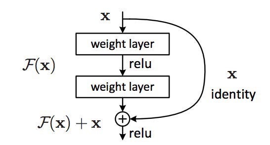ResNet block

Each “block” in ResNet consists of a series of layers and a “shortcut” connection adding the input of the block to its output. The “add” operation is performed element-wise, and if the input and output are of different sizes, zero-padding or projections (via 1x1 convolutions) can be used to create matching dimensions.

If we go back to our thought experiment, this simplifies our construction of identity layers greatly. Intuitively, it’s much easier to learn to push F(x) to 0 and leave the output as x than to learn an identity transformation from scratch. In general, ResNet gives layers a “reference” point — x — to start learning from.

This idea works astoundingly well in practice. Previously, deep neural nets often suffered from the problem of vanishing gradients, in which gradient signals from the error function decreased exponentially as they backpropogated to earlier layers. In essence, by the time the error signals traveled all the way back to the early layers, they were so small that the net couldn’t learn. However, because the gradient signal in ResNets could travel back directly to early layers via shortcut connections, we could suddenly build 50-layer, 101-layer, 152-layer, and even (apparently) 1000+ layer nets that still performed well. At the time, this was a huge leap forward from the previous state-of-the-art, which won the ILSVRC 2014 challenge with 22 layers.

ResNet is one of my personal favorite developments in the neural network world. So many deep learning papers come out with minor improvements from hacking away at the math, the optimizations, and the training process without thought to the underlying task of the model. ResNet fundamentally changed the way we understand neural networks and how they learn.

Fun facts:

• The 1000+ layer net is open-source! I would not really recommend you try re-training it, but…

• If you’re feeling functional and a little frisky, I recently ported ResNet50 to the open-source Clojure ML library Cortex. Try it out and see how it compares to Keras!

Inception

If ResNet was all about going deeper, the Inception Family™ is all about going wider. In particular, the authors of Inception were interested in the computational efficiency of training larger nets. In other words: how can we scale up neural nets without increasing computational cost?

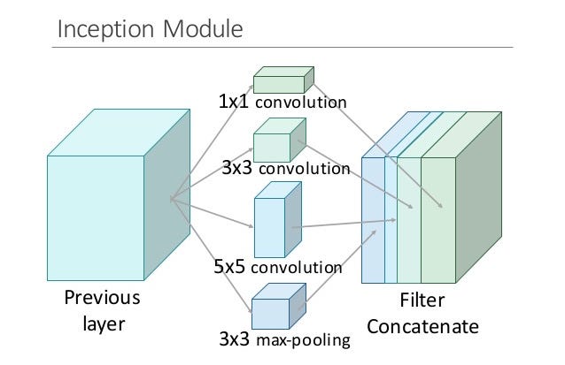
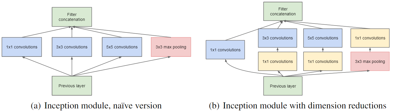
The original paper focused on a new building block for deep nets, a block now known as the “Inception module.” At its core, this module is the product of two key insights.

The first insight relates to layer operations. In a traditional conv net, each layer extracts information from the previous layer in order to transform the input data into a more useful representation. However, each layer type extracts a different kind of information. The output of a 5x5 convolutional kernel tells us something different from the output of a 3x3 convolutional kernel, which tells us something different from the output of a max-pooling kernel, and so on and so on. At any given layer, how do we know what transformation provides the most “useful” information?

Insight #1: why not let the model choose?

An Inception module computes multiple different transformations over the same input map* in parallel, concatenating their results into a single output. In other words, for each layer, Inception does a 5x5 convolutional transformation, *and a 3x3, and a max-pool. And the next layer of the model gets to decide if (and how) to use each piece of information.

The increased information density of this model architecture comes with one glaring problem: we’ve drastically increased computational costs. Not only are large (e.g. 5x5) convolutional filters inherently expensive to compute, stacking multiple different filters side by side greatly increases the number of feature maps per layer. And this increase becomes a deadly bottleneck in our model.

Think about it this way. For each additional filter added, we have to convolve over all the input maps to calculate a single output. See the image below: creating one output map from a single filter involves computing over every single map from the previous layer.

Let’s say there are M input maps. One additional filter means convolving over M more maps; N additional filters means convolving over NM more maps. In other words, as the authors note, “any uniform increase in the number of [filters] results in a quadratic increase of computation.” Our naive Inception module just tripled or quadrupled the number of filters. Computationally speaking, this is a Big Bad Thing.

This leads to insight #2: using 1x1 convolutions to perform dimensionality reduction. In order to solve the computational bottleneck, the authors of Inception used 1x1 convolutions to “filter” the depth of the outputs. A 1x1 convolution only looks at one value at a time, but across multiple channels, it can extract spatial information and compress it down to a lower dimension. For example, using 20 1x1 filters, an input of size 64x64x100 (with 100 feature maps) can be compressed down to 64x64x20. By reducing the number of input maps, the authors of Inception were able to stack different layer transformations in parallel, resulting in nets that were simultaneously deep (many layers) and “wide” (many parallel operations).

How well did this work? The first version of Inception, dubbed “GoogLeNet,” was the 22-layer winner of the ILSVRC 2014 competition I mentioned earlier. Inception v2 and v3 were developed in a second paper a year later, and improved on the original in several ways — most notably by refactoring larger convolutions into consecutive smaller ones that were easier to learn. In v3, for example, the 5x5 convolution was replaced with 2 consecutive 3x3 convolutions.

Inception rapidly became a defining model architecture. The latest version of Inception, v4, even threw in residual connections within each module, creating an Inception-ResNet hybrid. Most importantly, however, Inception demonstrated the power of well-designed “network-in-network” architectures, adding yet another step to the representational power of neural networks.

Fun facts:

• The original Inception paper literally cites the “we need to go deeper” internet meme as an inspiration for its name. This must be the first time knowyourmeme.com got listed as the first reference of a Google paper.

• The second Inception paper (with v2 and v3) was released just one day after the original ResNet paper. December 2015 was a good time for deep learning.

Xception

Xception stands for “extreme inception.” Rather like our previous two architectures, it reframes the way we look at neural nets — conv nets in particular. And, as the name suggests, it takes the principles of Inception to an extreme.

Here’s the hypothesis: “cross-channel correlations and spatial correlations are sufficiently decoupled that it is preferable not to map them jointly.”

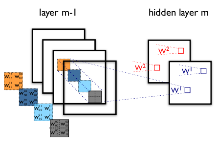
What does this mean? Well, in a traditional conv net, convolutional layers seek out correlations across both space and depth. Let’s take another look at our standard convolutional layer:

In the image above, the filter simultaneously considers a spatial dimension (each 2x2 colored square) and a cross-channel or “depth” dimension (the stack of four squares). At the input layer of an image, this is equivalent to a convolutional filter looking at a 2x2 patch of pixels across all three RGB channels. Here’s the question: is there any reason we need to consider both the image region and the channels at the same time?

In Inception, we began separating the two slightly. We used 1x1 convolutions to project the original input into several separate, smaller input spaces, and from each of those input spaces we used a different type of filter to transform those smaller 3D blocks of data. Xception takes this one step further. Instead of partitioning input data into several compressed chunks, it maps the spatial correlations for each output channel separately, and then performs a 1x1 depthwise convolution to capture cross-channel correlation.

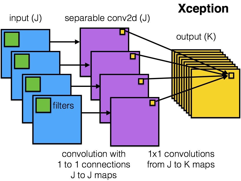
The author notes that this is essentially equivalent to an existing operation known as a “depthwise separable convolution,” which consists of a depthwise convolution (a spatial convolution performed independently for each channel) followed by a pointwise convolution (a 1x1 convolution across channels). We can think of this as looking for correlations across a 2D space first, followed by looking for correlations across a 1D space. Intuitively, this 2D + 1D mapping is easier to learn than a full 3D mapping.

And it works! Xception slightly outperforms Inception v3 on the ImageNet dataset, and vastly outperforms it on a larger image classification dataset with 17,000 classes. Most importantly, it has the same number of model parameters as Inception, implying a greater computational efficiency. Xception is much newer (it came out in April 2017), but as mentioned above, its architecture is already powering Google’s mobile vision applications through MobileNet.

Fun facts:

• The author of Xception is also the author of Keras. Francois Chollet is a living god.

Moving forward

That’s it for ResNet, Inception, and Xception! I firmly believe in having a strong intuitive understanding of these networks, because they are becoming ubiquitous in research and industry alike. We can even use them in our own applications with something called transfer learning.

Transfer learning is a technique in machine learning in which we apply knowledge from a source domain (e.g. ImageNet) to a target domain that may have significantly fewer data points. In practice, this generally involves initializing a model with pre-trained weights from ResNet, Inception, etc. and either using it as a feature extractor, or fine-tuning the last few layers on a new dataset. With transfer learning, these models can be re-purposed for any related task we want, from object detection for self-driving vehicles to generating captions for video clips.

To get started with transfer learning, Keras has a wonderful guide to fine-tuning models here. If it sounds interesting to you, check it out — and happy hacking!