With the rise of autonomous vehicles, smart video surveillance, facial detection and various people counting applications, fast and accurate object detection systems are rising in demand. These systems involve not only recognizing and classifying every object in an image, but localizing each one by drawing the appropriate bounding box around it. This makes object detection a significantly harder task than its traditional computer vision predecessor, image classification.

Fortunately, however, the most successful approaches to object detection are currently extensions of image classification models. A few months ago, Google released a new object detection API for Tensorflow. With this release came the pre-built architectures and weights for a few specific models:

• Single Shot Multibox Detector (SSD) with MobileNets

• SSD with Inception V2

• Region-Based Fully Convolutional Networks (R-FCN) with Resnet 101

• Faster RCNN with Resnet 101

• Faster RCNN with Inception Resnet v2

In my last blog post, I covered the intuition behind the three base network architectures listed above: MobileNets, Inception, and ResNet. This time around, I want to do the same for Tensorflow’s object detection models: Faster R-CNN, R-FCN, and SSD. By the end of this post, we will hopefully have gained an understanding of how deep learning is applied to object detection, and how these object detection models both inspire and diverge from one another.

Faster R-CNN

Faster R-CNN is now a canonical model for deep learning-based object detection. It helped inspire many detection and segmentation models that came after it, including the two others we’re going to examine today. Unfortunately, we can’t really begin to understand Faster R-CNN without understanding its own predecessors, R-CNN and Fast R-CNN, so let’s take a quick dive into its ancestry.

R-CNN

R-CNN is the grand-daddy of Faster R-CNN. In other words, R-CNN really kicked things off.

R-CNN, or Region-based Convolutional Neural Network, consisted of 3 simple steps:

1. Scan the input image for possible objects using an algorithm called Selective Search, generating ~2000 region proposals

2. Run a convolutional neural net (CNN) on top of each of these region proposals

3. Take the output of each CNN and feed it into a) an SVM to classify the region and b) a linear regressor to tighten the bounding box of the object, if such an object exists.

These 3 steps are illustrated in the image below:

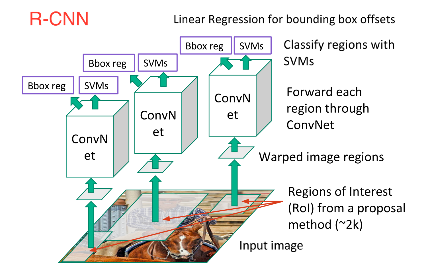
In other words, we first propose regions, then extract features, and then classify those regions based on their features. In essence, we have turned object detection into an image classification problem. R-CNN was very intuitive, but very slow.

Fast R-CNN

R-CNN’s immediate descendant was Fast-R-CNN. Fast R-CNN resembled the original in many ways, but improved on its detection speed through two main augmentations:

1. Performing feature extraction over the image before proposing regions, thus only running one CNN over the entire image instead of 2000 CNN’s over 2000 overlapping regions

2. Replacing the SVM with a softmax layer, thus extending the neural network for predictions instead of creating a new model

The new model looked something like this:

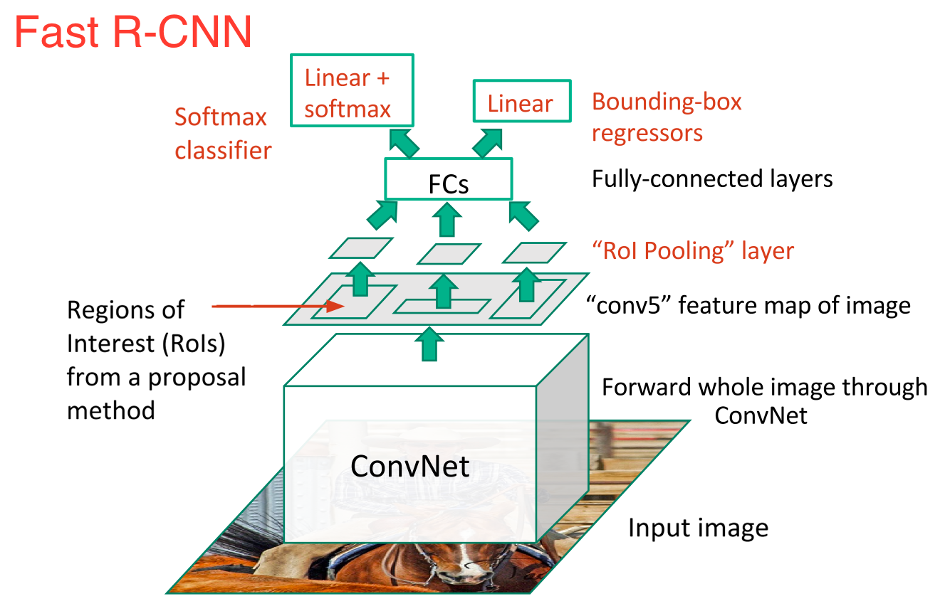
As we can see from the image, we are now generating region proposals based on the last feature map of the network, not from the original image itself. As a result, we can train just one CNN for the entire image.

In addition, instead of training many different SVM’s to classify each object class, there is a single softmax layer that outputs the class probabilities directly. Now we only have one neural net to train, as opposed to one neural net and many SVM’s.

Fast R-CNN performed much better in terms of speed. There was just one big bottleneck remaining: the selective search algorithm for generating region proposals.

Faster R-CNN

At this point, we’re back to our original target: Faster R-CNN. The main insight of Faster R-CNN was to replace the slow selective search algorithm with a fast neural net. Specifically, it introduced the region proposal network (RPN).

Here’s how the RPN worked:

• At the last layer of an initial CNN, a 3x3 sliding window moves across the feature map and maps it to a lower dimension (e.g. 256-d)

• For each sliding-window location, it generates multiple possible regions based on k fixed-ratio anchor boxes (default bounding boxes)

• Each region proposal consists of a) an “objectness” score for that region and b) 4 coordinates representing the bounding box of the region

In other words, we look at each location in our last feature map and consider k different boxes centered around it: a tall box, a wide box, a large box, etc. For each of those boxes, we output whether or not we think it contains an object, and what the coordinates for that box are. This is what it looks like at one sliding window location:

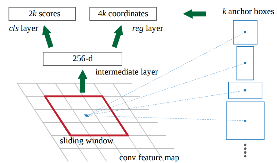
The 2k scores represent the softmax probability of each of the k bounding boxes being on “object.” Notice that although the RPN outputs bounding box coordinates, it does not try to classify any potential objects: its sole job is still proposing object regions. If an anchor box has an “objectness” score above a certain threshold, that box’s coordinates get passed forward as a region proposal.

Once we have our region proposals, we feed them straight into what is essentially a Fast R-CNN. We add a pooling layer, some fully-connected layers, and finally a softmax classification layer and bounding box regressor. In a sense, Faster R-CNN = RPN + Fast R-CNN.

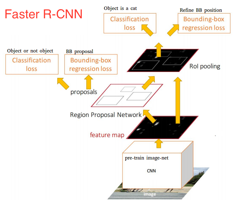
Altogether, Faster R-CNN achieved much better speeds and a state-of-the-art accuracy. It is worth noting that although future models did a lot to increase detection speeds, few models managed to outperform Faster R-CNN by a significant margin. In other words, Faster R-CNN may not be the simplest or fastest method for object detection, but it is still one of the best performing. Case in point, Tensorflow’s Faster R-CNN with Inception ResNet is their slowest but most accurate model.

At the end of the day, Faster R-CNN may look complicated, but its core design is the same as the original R-CNN: hypothesize object regions and then classify them. This is now the predominant pipeline for many object detection models, including our next one.

R-FCN

Remember how Fast R-CNN improved on the original’s detection speed by sharing a single CNN computation across all region proposals? That kind of thinking was also the motivation behind R-FCN: increase speed by maximizing shared computation.

R-FCN, or Region-based Fully Convolutional Net, shares 100% of the computations across every single output. Being fully convolutional, it ran into a unique problem in model design.

On the one hand, when performing classification of an object, we want to learn location invariance in a model: regardless of where the cat appears in the image, we want to classify it as a cat. On the other hand, when performing detection of the object, we want to learn location variance: if the cat is in the top left-hand corner, we want to draw a box in the top left-hand corner. So if we’re trying to share convolutional computations across 100% of the net, how do we compromise between location invariance and location variance?

R-FCN’s solution: position-sensitive score maps.

Each position-sensitive score map represents one relative position of one object class. For example, one score map might activate wherever it detects the top-right of a cat. Another score map might activate where it sees the bottom-left of a car. You get the point. Essentially, these score maps are convolutional feature maps that have been trained to recognize certain parts of each object.

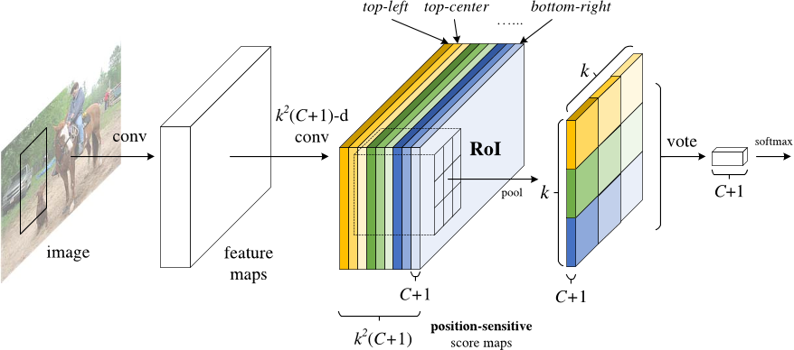
Now, R-FCN works as follows:

1. Run a CNN (in this case, ResNet) over the input image

2. Add a fully convolutional layer to generate a score bank of the aforementioned “position-sensitive score maps.” There should be k²(C+1) score maps, with k² representing the number of relative positions to divide an object (e.g. 3² for a 3 by 3 grid) and C+1 representing the number of classes plus the background.

3. Run a fully convolutional region proposal network (RPN) to generate regions of interest (RoI’s)

4. For each RoI, divide it into the same k² “bins” or subregions as the score maps

5. For each bin, check the score bank to see if that bin matches the corresponding position of some object. For example, if I’m on the “upper-left” bin, I will grab the score maps that correspond to the “upper-left” corner of an object and average those values in the RoI region. This process is repeated for each class.

6. Once each of the k² bins has an “object match” value for each class, average the bins to get a single score per class.

7. Classify the RoI with a softmax over the remaining C+1 dimensional vector

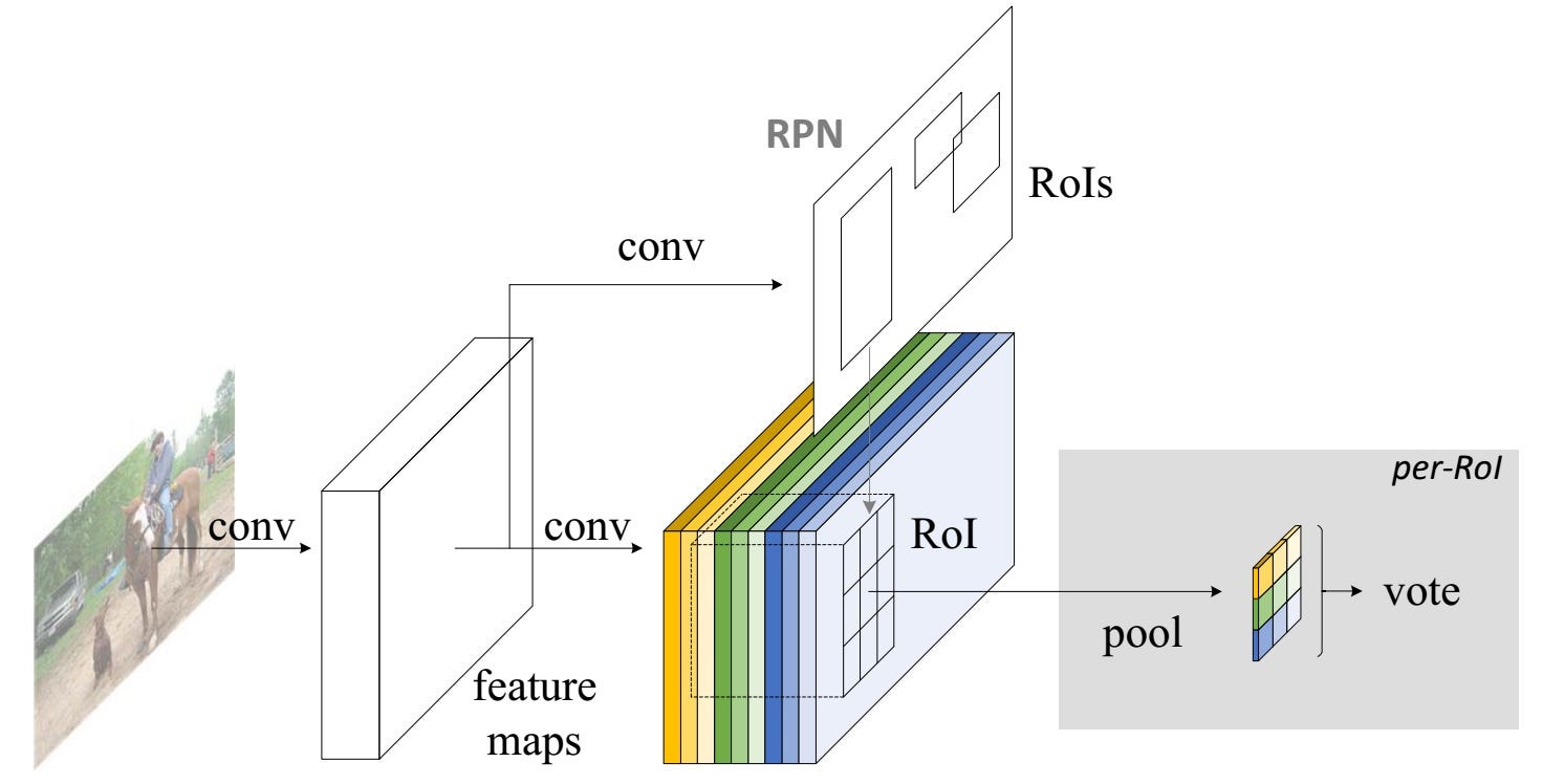
Altogether, R-FCN looks something like this, with an RPN generating the RoI’s:

Even with the explanation and the image, you might still be a little confused on how this model works. Honestly, R-FCN is much easier to understand when you can visualize what it’s doing. Here is one such example of an R-FCN in practice, detecting a baby:

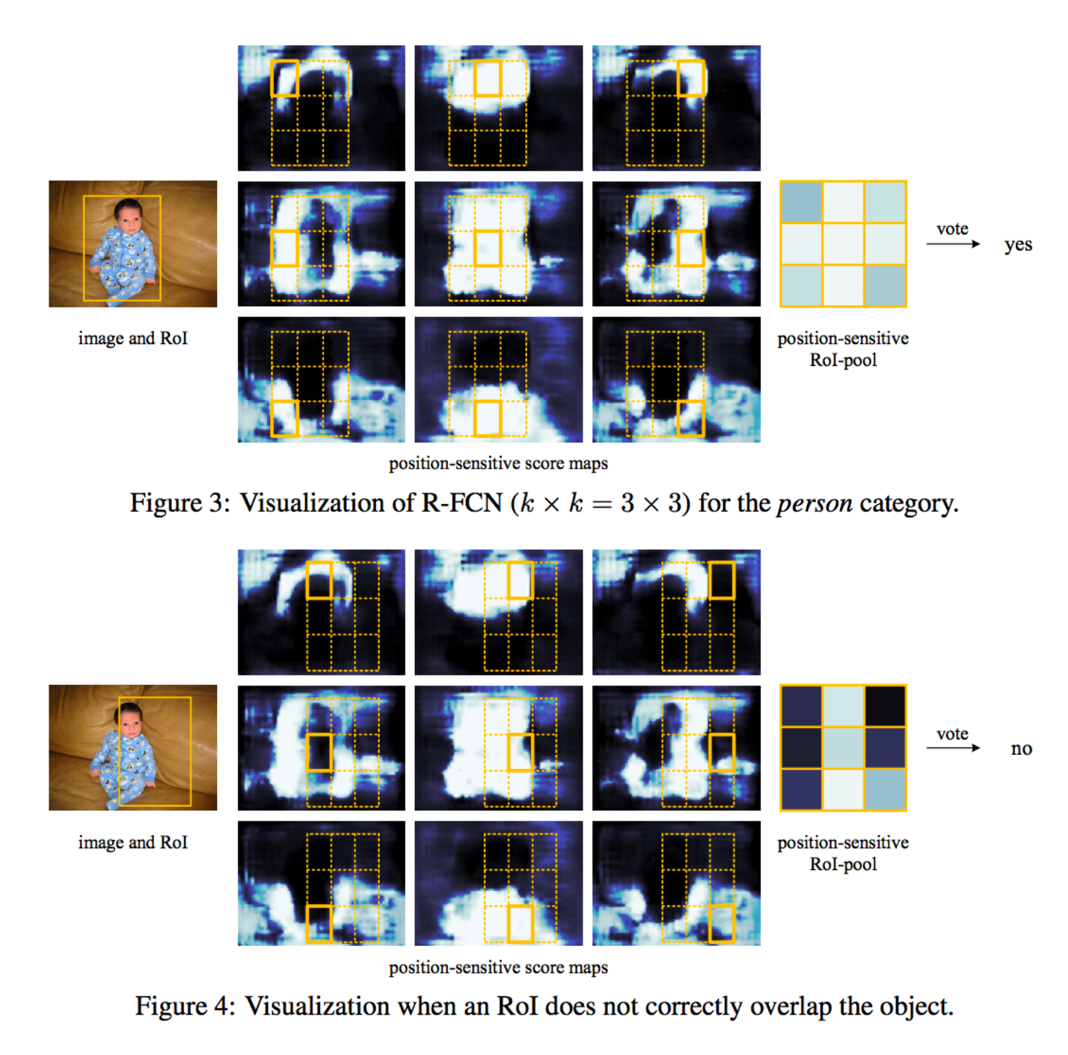
Simply put, R-FCN considers each region proposal, divides it up into sub-regions, and iterates over the sub-regions asking: “does this look like the top-left of a baby?”, “does this look like the top-center of a baby?” “does this look like the top-right of a baby?”, etc. It repeats this for all possible classes. If enough of the sub-regions say “yes, I match up with that part of a baby!”, the RoI gets classified as a baby after a softmax over all the classes.

With this setup, R-FCN is able to simultaneously address location variance *by proposing different object regions, and *location invariance by having each region proposal refer back to the same bank of score maps. These score maps should learn to classify a cat as a cat, regardless of where the cat appears. Best of all, it is fully convolutional, meaning all of the computation is shared throughout the network.

As a result, R-FCN is several times faster than Faster R-CNN, and achieves comparable accuracy.

SSD

Our final model is SSD, which stands for Single-Shot Detector. Like R-FCN, it provides enormous speed gains over Faster R-CNN, but does so in a markedly different manner.

Our first two models performed region proposals and region classifications in two separate steps. First, they used a region proposal network to generate regions of interest; next, they used either fully-connected layers or position-sensitive convolutional layers to classify those regions. SSD does the two in a “single shot,” simultaneously predicting the bounding box and the class as it processes the image.

Concretely, given an input image and a set of ground truth labels, SSD does the following:

1. Pass the image through a series of convolutional layers, yielding several sets of feature maps at different scales (e.g. 10x10, then 6x6, then 3x3, etc.)

2. For each location in each of these feature maps, use a 3x3 convolutional filter to evaluate a small set of default bounding boxes. These default bounding boxes are essentially equivalent to Faster R-CNN’s anchor boxes.

3. For each box, simultaneously predict a) the bounding box offset and b) the class probabilities

4. During training, match the ground truth box with these predicted boxes based on IoU. The best predicted box will be labeled a “positive,” along with all other boxes that have an IoU with the truth >0.5.

SSD sounds straightforward, but training it has a unique challenge. With the previous two models, the region proposal network ensured that everything we tried to classify had some minimum probability of being an “object.” With SSD, however, we skip that filtering step. We classify and draw bounding boxes from every single position in the image, using multiple different shapes, at several different scales. As a result, we generate a much greater number of bounding boxes than the other models, and nearly all of the them are negative examples.

To fix this imbalance, SSD does two things. Firstly, it uses non-maximum suppression to group together highly-overlapping boxes into a single box. In other words, if four boxes of similar shapes, sizes, etc. contain the same dog, NMS would keep the one with the highest confidence and discard the rest. Secondly, the model uses a technique called hard negative mining to balance classes during training. In hard negative mining, only a subset of the negative examples with the highest training loss (i.e. false positives) are used at each iteration of training. SSD keeps a 3:1 ratio of negatives to positives.

Its architecture looks like this:

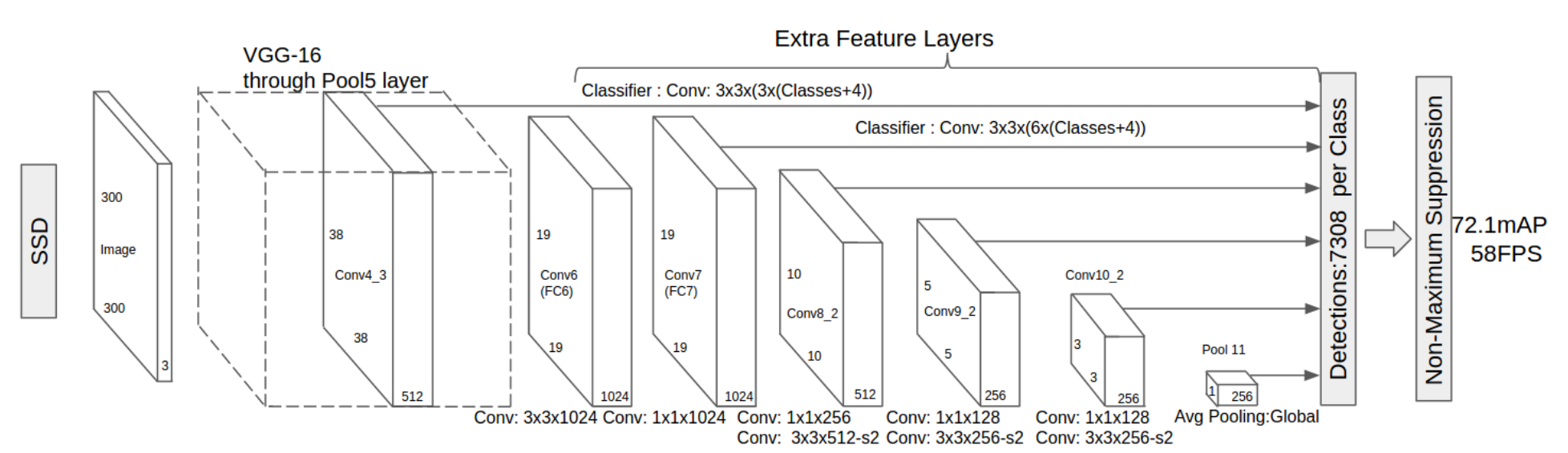
As I mentioned above, there are “extra feature layers” at the end that scale down in size. These varying-size feature maps help capture objects of different sizes. For example, here is SSD in action:

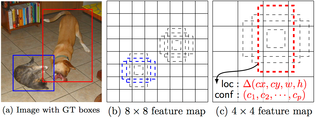
In smaller feature maps (e.g. 4x4), each cell covers a larger region of the image, enabling them to detect larger objects. Region proposal and classification are performed simultaneously: given p object classes, each bounding box is associated with a (4+p)-dimensional vector that outputs 4 box offset coordinates and p class probabilities. In the last step, softmax is again used to classify the object.

Ultimately, SSD is not so different from the first two models. It simply skips the “region proposal” step, instead considering every single bounding box in every location of the image simultaneously with its classification. Because SSD does everything in one shot, it is the fastest of the three models, and still performs quite comparably.

Conclusion

Faster R-CNN, R-FCN, and SSD are three of the best and most widely used object detection models out there right now. Other popular models tend to be fairly similar to these three, all relying on deep CNN’s (read: ResNet, Inception, etc.) to do the initial heavy lifting and largely following the same proposal/classification pipeline.

At this point, putting these models to use just requires knowing Tensorflow’s API. Tensorflow has a starter tutorial on using these models here. Give it a try, and happy hacking!