One of my favorite things about deep reinforcement learning is that, unlike supervised learning, it really, really doesn’t want to work. Throwing a neural net at a computer vision problem might get you 80% of the way there. Throwing a neural net at an RL problem will probably blow something up in front of your face — and it will blow up in a different way each time you try.

A lot of the biggest challenges in RL revolve around two questions: how we interact with the environment effectively (e.g. exploration vs. exploitation, sample efficiency), and how we learn from experience effectively (e.g. long-term credit assignment, sparse reward signals). In this post, I want to explore a few recent directions in deep RL research that attempt to address these challenges, and do so with particularly elegant parallels to human cognition. In particular, I want to talk about:

• hierarchical RL,

• memory and predictive modeling, and

• combined model-free and model-based approaches.

This post will begin with a quick review of two canonical deep RL algorithms — DQN and A3C — to provide us some intuitions to refer back to, and then jump into a deep dive on a few recent papers and breakthroughs in the categories described above.

Review: DQN and A3C/A2C

Disclaimer: I am assuming some basic familiarity with RL (and thus will not provide an in-depth tutorial on either of these algorithms), but even if you’re not 100% solid on how they work, the rest of the post should still be accessible.

DeepMind’s DQN (deep Q-network) was one of the first breakthrough successes in applying deep learning to RL. It used a neural net to learn Q-functions for classic Atari games such as Pong and Breakout, allowing the model to go straight from raw pixel input to an action.

Algorithmically, the DQN draws directly on classic Q-learning techniques. In Q-learning, the Q-value, or “quality”, of a state-action pair is estimated through iterative updates based on experience. In essence, with every action we take in a state, we can use the immediate reward we receive and a value estimate of our new state to update the value estimate of our original state-action pair:

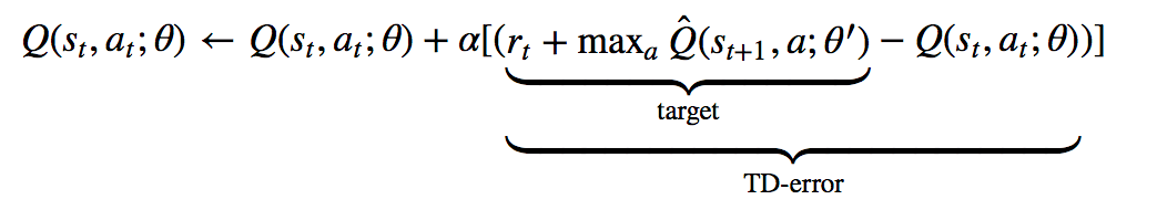
Training DQN consists of minimizing the MSE (mean squared error) of the Temporal Difference error, or TD-error, which is shown above. The two key strategies employed by DQN to adapt Q-learning for deep neural nets, which have since been successfully adopted by many subsequent deep RL efforts, were:

• experience replay, in which each state/action transition tuple (s, a, r, s’) is stored in a memory “replay” buffer and randomly sampled to train the network, allowing for re-use of training data and de-correlation of consecutive trajectory samples; and

• use of a separate target network — the Q_hat part of the above equation — to stabilize training, so the TD error isn’t being calculated from a constantly changing target from the training network, but rather from a stable target generated by a mostly fixed network.

Subsequently, DeepMind’s A3C (Asynchronous Advantage Actor Critic) and OpenAI’s synchronous variant A2C, popularized a very successful deep learning-based approach to actor-critic methods.

Actor-critic methods combine policy gradient methods with a** learned value function*. With DQN, we only had the learned value function — the Q-function — and the “policy” we followed was simply taking the action that maximized the Q-value at each step. With A3C, as with the rest of actor-critic methods, we learn two different functions: the policy (or “actor”), and the value (the “critic”). The policy adjusts action probabilities based on the current estimated *advantage of taking that action, and the value function updates that advantage based on the experience and rewards collected by following the policy:

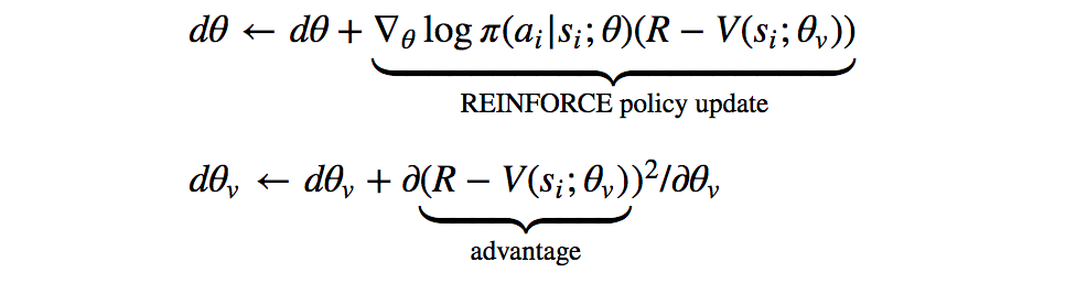
As we can see from the updates above, the value network learns a baseline state value V(s_i;θ_v) with which we can compare our current reward estimate, R, to obtain the “advantage,” and the policy network adjusts the log probabilities of actions based on that advantage via the classic REINFORCE algorithm.

The real contribution of A3C comes from its parallelized and asynchronous architecture: multiple actor-learners are dispatched to separate instantiations of the environment; they all interact with the environment and collect experience, and asynchronously push their gradient updates to a central “target network” (an idea borrowed from DQN). Later, OpenAI showed with A2C that asynchronicity does not actually contribute to performance, and in fact reduces sample efficiency. Unfortunately, details of these architectures are beyond the scope of this post, but if distributed agents excite you like they excite me, make sure you check out DeepMind’s IMPALA — very useful design paradigm for scaling up learning.

Both DQN and A3C/A2C can be powerful baseline agents, but they tend to suffer when faced with more complex tasks, severe partial observability, and/or long delays between actions and relevant reward signals. As a result, entire subfields of RL research have emerged to address these issues. Let’s get into some of the good stuff :).

Hierarchical Reinforcement Learning

Hierarchical RL is a class of reinforcement learning methods that learns from multiple layers of policy, each of which is responsible for control at a different level of temporal and behavioral abstraction. The lowest level of policy is responsible for outputting environment actions, leaving higher levels of policy free to operate over more abstract goals and longer timescales.

Why is this so appealing? First and foremost, on the cognitive front, research has long suggested that human and animal behavior is underpinned by hierarchical structure. This is intuitive in everyday life: when I decide to cook a meal (which is basically never, by the way, but for the sake of argument let us assume I am a responsible human being), I am able to divide this task into simpler sub-tasks: chopping vegetables, boiling pasta, etc. without losing sight of my overarching goal of cooking a meal; I am even able to swap out sub-tasks, e.g. cooking rice instead of making pasta, to complete the same goal. This suggests an inherent hierarchy and compositionality in real-world tasks, in which simple, atomic actions can be strung together, repeated, and composed to complete complicated jobs. In recent years, research has even uncovered direct parallels between HRL components and specific neural structures within the prefrontal cortex.

On the technical RL front, HRL is especially appealing because it helps address two of the biggest challenges I mentioned under our second question, i.e. how to learn from experience effectively: long-term credit assignment and sparse reward signals. In HRL, because low-level policies learn from intrinsic rewards based on tasks assigned by high-level policies, atomic tasks can still be learned in spite of sparse rewards. Furthermore, the temporal abstraction developed by high-level policies enables our model to handle credit assignment over temporally extended experiences.

So how does it work? There are a number of different ways to implement HRL. One recent paper from Google Brain takes a particularly clean and simple approach, and introduces some nice off-policy corrections for data-efficient training. Their model is called HIRO.

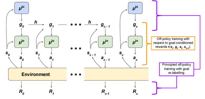μ_hi is the high-level policy, which outputs “goal states” for the low-level policy to reach. μ_lo, the low-level policy, outputs environment actions in an attempt to reach that goal state observation.

Here’s the idea: we have 2 layers of policy. The high-level policy is trained to maximize the environment reward R. Every c timesteps, the high-level policy samples a new action, which is a “goal state” for the low-level policy to reach. The low-level policy is trained to take environment actions that would produce a state observation similar to the given goal state.

Consider a simple example: say we are training a robot to stack colored cubes in a certain order. We only get a single reward of +1 in the end if the task is completed successfully, and a reward of 0 at all other time-steps. Intuitively, the high-level policy is responsible for coming up with the necessary sub-goals to complete: perhaps the first goal state it outputs would be “observe a red cube in front of you;” the next might be “observe a blue cube next to a red cube;” and then “observe a blue cube on top of a red cube.” The low-level policy bumbles around the environment until it comes up with the sequence of actions necessary to produce these observations, e.g. picking up the blue cube and moving it on top of the red one.

HIRO uses a variant of the DDPG (Deep Deterministic Policy Gradient) training objective to train the low-level policy, whose intrinsic reward is parameterized as the distance between the current observation and the goal observation:

DDPG is another seminal deep RL algorithm that extended ideas from DQN to a continuous action space. It is another actor-critic method that uses policy gradients to optimize the policy, but instead of optimizing it with respect to the advantage as in A3C, it optimizes it with respect to the Q-values. Thus in HIRO, the DDPG-adjacent error to minimize becomes:

Meanwhile, in order to use off-policy experience, the high-level policy is trained with off-policy corrections. Here’s the idea: to be sample efficient, we want to use some form of replay buffer, like DQN. However, old experience cannot be used directly to train the high-level policy. This is because the low-level policy is constantly learning and changing, so even if we condition on the same goals as our old experience, our low-level policy may now exhibit different actions/transitions. The off-policy correction proposed in HIRO is to retroactively change the goal seen in off-policy experience to maximize the likelihood of the observed action sequence. In other words, if the replay experience says the old agent took actions (x,y,z) to reach goal g, we find a goal g̃ that would make the current agent most likely to take those same actions (x,y,z), i.e. one that would maximize this log probability of the action sequence:

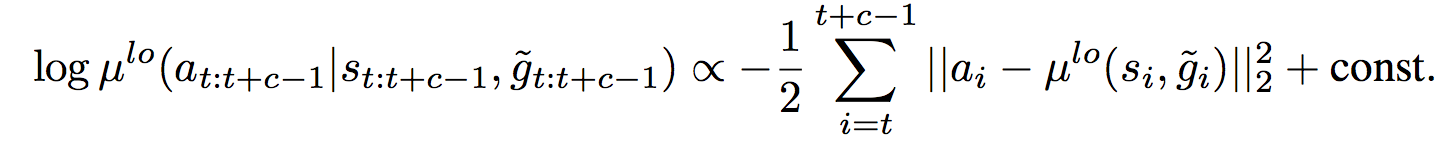
The high-level policy is then trained with a DDPG variant on those actions, the new goal, and the environment reward R.

HIRO is certainly not the only approach to HRL. FeUdal networks were an earlier, related work that used a learned “goal” representation instead of the raw state observation. Indeed, lot of variation in research stems from different ways to learn useful low-level sub-policies; many papers have used auxiliary or “proxy” rewards, and others have experimented with pre-training or multi-task training. Unlike HIRO, many of these approaches require some degree of hand engineering or domain knowledge, which inherently limits generalizability. Another recently-explored option is to use population-based training (PBT), another algorithm I am a personal fan of. In essence, internal rewards are treated as additional hyperparameters, and PBT learns the optimal evolution of these hyperparameters across “evolving” populations during training.

HRL is a very popular area of research right now, and is very easily interpolatable with other techniques (check out this paper combining HRL with imitation learning). At its core, however, it’s just a really intuitive idea. It’s extensible, has neuroanatomical parallels, and addresses a bunch of fundamental problems in RL. Like the rest of good RL, though, it can be quite tricky to train.

Memory and Attention

Now let’s talk about some other ways to address the problems of long-term credit assignment and sparse reward signals. Specifically, let’s talk about the most obvious way: make the agent really good at remembering things.

Memory in deep learning is always fun, because try as researchers might (and really, they do try), few architectures beat out a well-tuned LSTM. Human memory, however, does not work anything like an LSTM; when we go about tasks in daily life, we recall and attend to specific, context-dependent memories, and little else. When I go back home and drive to the local grocery store, I’m using memories from the last hundred times I’ve driven this route, not memories of how to get from Camden Town to Piccadilly Circus in London — even if those memories are fresh in recent experience. In this sense, our memory almost seems queryable by context: depending on where I am and what I’m doing, my brain knows which memories will be useful to me.

In deep learning, this is the driving thesis behind external, key-value-based memory stores. This idea is not new; Neural Turing Machines, one of the first and favorite papers I ever read, augmented neural nets with a differentiable, external memory store accessible via vector-valued “read” and “write” heads to specific locations. We can easily imagine this being extended into RL, where at any given time-step, an agent is given both its environment observation and memories relevant to its current state. That’s exactly what the recent MERLIN architecture extends upon.

MERLIN has 2 components: a memory-based predictor (MBP), and a policy network. The MBP is responsible for compressing observations into useful, low-dimensional “state variables” to store directly into a key-value memory matrix. It is also responsible for passing relevant memories to the policy, which uses those memories and the current state to output actions.

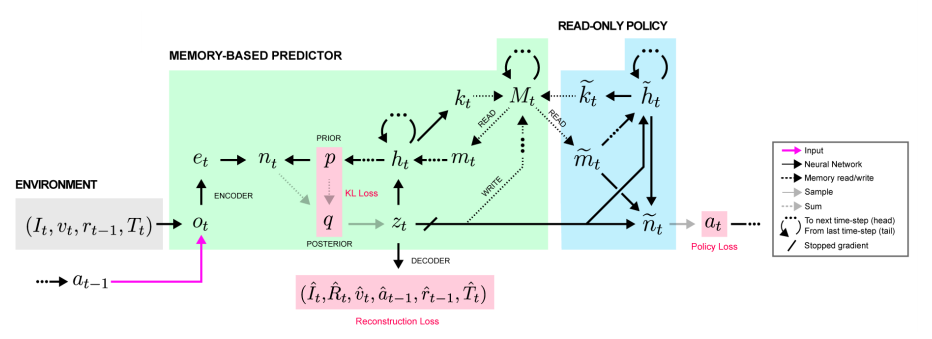
This architecture may look a little complicated, but remember, the policy is just an recurrent net outputting actions, and the MBP is only really doing 3 things:

• compressing the observation into a useful state variable z_t to pass on to the policy,

• writing z_t into a memory matrix, and

• fetching other useful memories to pass on to the policy.

The pipeline looks something like this: the input observation is first encoded and then fed through an MLP, the output of which is added to the prior distribution over the next state variable to produce the posterior distribution. This posterior distribution, which is conditioned on all the previous actions/observations as well as this new observation, is then sampled to produce a state variable z_t. Next, z_t gets fed into the MBP’s LSTM, whose output is used to update the prior and to read to/write from memory via vector-valued “read keys” and “write keys” — both of which are produced as a linear function of the LSTM’s hidden state. Finally, downstream, the policy net leverages both z_t and read outputs from memory to produce an action.

A key detail is that in order to ensure the state representations are useful, the MBP is also trained to predict the reward from the current state z_t, so learned representations are relevant to the task at hand.

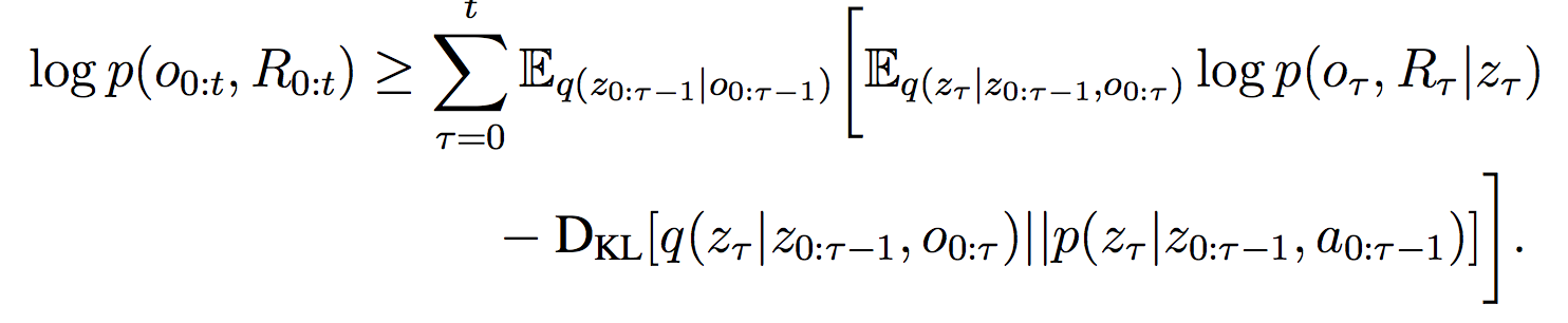
Training of MERLIN is a bit complicated; since the MBP is intended to serve as a useful “world model,” an intractable objective, it is trained to optimize the variational lower bound (VLB) loss instead. (If you are unfamiliar with VLB, I found this post quite useful, but you really don’t need it to understand MERLIN). There are two components to this VLB loss:

1. The KL-divergence between the prior and posterior probability distributions over this next state variable, where the posterior is additionally conditioned on the new observation. Minimizing this KL ensures that this new state variable is consistent with previous observations/actions.

2. The reconstruction loss of the state variable, in which we attempt to reproduce the input observation (e.g. the image, previous action, etc.) and predict the reward based on the state variable. If this loss is small, we have found a state variable that is an accurate representation of the observation, and useful for producing actions that give a high reward.

Here is our final VLB loss, with the first term being reconstruction and the second being the KL divergence:

The policy network’s loss is a slightly fancier version of the policy gradient loss we discussed above with A3C; it uses an algorithm called the Generalized Advantage Estimation Algorithm, the details of which are beyond the scope of this post (but can be found in section 4.4 of the MERLIN paper’s appendix), but it looks similar to the standard policy gradient update shown below:

Once trained, MERLIN should be able to predictively model the world through state representations and memory, and its policy should be able to leverage those predictions to take useful actions.

MERLIN is not the only deep RL work to use external memory stores — all the way back in 2016, researchers were already applying this idea in an MQN, or Memory Q-Network, to solve mazes in Minecraft — but this concept of using memory as a predictive model of the world has some unique neuroscientific traction. Another Medium post has done a great job of exploring this idea, so I won’t repeat it all here, but the key argument is that our brain likely does not function as an “input-output” machine, like most neural nets are interpreted. Instead, it functions as a prediction engine, and our perception of the world is actually just the brain’s best guesses about the causes of our sensory inputs. Neuroscientist Amil Seth sums up this 19th century theory by Hermann von Helmholtz nicely:

The brain is locked inside a bony skull. All it receives are ambiguous and noisy sensory signals that are only indirectly related to objects in the world. Perception must therefore be a process of inference, in which indeterminate sensory signals are combined with prior expectations or ‘beliefs’ about the way the world is, to form the brain’s optimal hypotheses of the causes of these sensory signals.

MERLIN’s memory-based predictor aims to fulfill this very purpose of predictive inference. It encodes observations and combines them with internal priors to generate a “state variable” that captures some representation — or cause — of the input, and stores these states in long-term memory so the agent can act upon them later.

Agents, World Models, and Imagination

Interestingly, the concept of the brain as a predictive engine actually leads us back to the first RL question we want to explore: how do we learn from the environment effectively? After all, if we’re not going straight from observations to actions, how should we best interact with and learn from the world around us?

Traditionally in RL, we can either do model-free learning or model-based learning. In model-free RL, we learn to map raw environment observations directly to values or actions. In model-based RL, we first learn a transition model of the environment based on raw observations, and then use that model to choose actions.

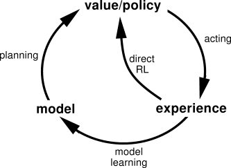The outside circle depicts model-based RL; the “direct RL” loop depicts model-free RL

Being able to plan based on a model is much more sample-efficient than having to work from pure trial-and-error as in model-free learning. However, learning a good model is often very difficult, and compounding errors from model imperfections generally leads to poor agent performance. For this reason, a lot of early successes in deep RL (e.g. DQN and A3C) were model-free.

That said, the lines between model-free and model-based RL have been blurred as early as the Dyna algorithm in 1990, in which a learned model is used to generate simulated experience to help train the model-free policy. Now in 2018, a new “Imagination-augmented Agents” algorithm has been introduced that directly combines the two approaches.

In Imagination-Augmented Agents (I2A), the final policy is a function of both a model-free component and a model-based component. The model-based component is referred to as the agent’s “imagination” of the world, and consists of imagined trajectories rolled out by the agent’s internal, learned model. The key, however, is that the model-based component also has an encoder at the end that aggregates the imagined trajectories and interprets them, enabling the agent to learn to ignore its imagination when necessary. In this sense, if the agent discovers its internal model is projecting useless and inaccurate trajectories, it can learn to ignore the model and proceed with its model-free arm.

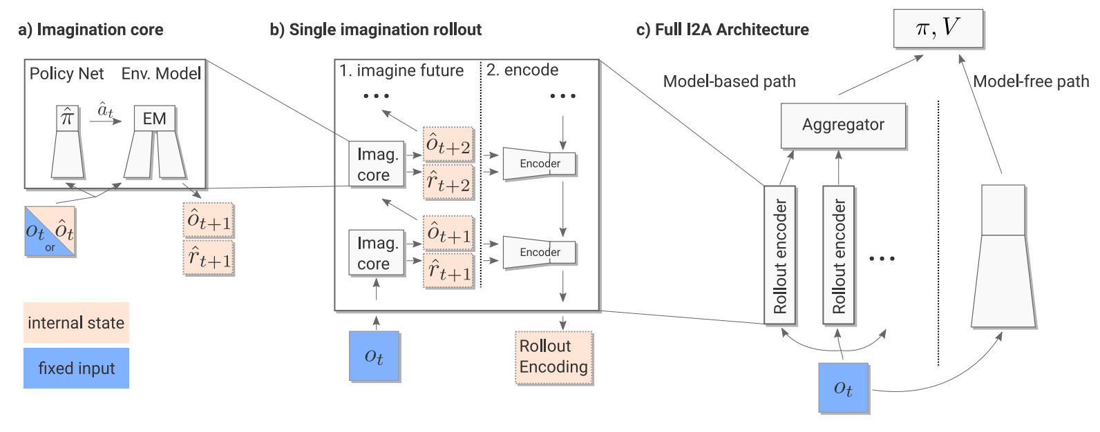
The figure above describes how I2A’s work. An observation is first passed to both the model-free and model-based components. In the model-based component, n different trajectories are “imagined” based on the n possible actions that could be taken in the current state. These trajectories are obtained by feeding the action and state into the internal environment model, transitioning to a new imagined state, taking the maximum next action in that, and so on. A distilled imagination policy (which is kept similar to the final policy via cross-entropy loss) chooses the next actions. After some fixed k steps, these trajectories are encoded and aggregated together, and fed into the policy network along with the output of the model-free component. Critically, the encoding allows the policy to interpret the imagined trajectories in whatever way is most useful — ignoring them if appropriate, extracting non-reward-related information when available, and so on.

The policy is trained via a standard policy gradient loss with advantage, similar to A3C and MERLIN, so this should look familiar by now:

Additionally, a policy distillation loss is added between the actual policy and the internal model’s imagined policy, to ensure that the imagined policy chooses actions similar to what the current agent would:

I2A outperforms a number of baselines, including the MCTS (Monte Carlo Tree Search) planning algorithm. It is also able to perform well in experiments where its model-based component is intentionally restricted to make poor predictions, demonstrating that it is able to trade-off use of the model in favor of model-free methods when necessary. Interestingly, the I2A with a poor internal model actually slightly outperformed the I2A with a good model in the end — the authors chalked this up to either random initialization or the noisy internal model providing some form of regularization in the end, but this is definitely an area for further investigation.

Regardless, the I2A is fascinating because it is, in some ways, also exactly how we go about acting in the world. We’re always planning and projecting into the future based on some mental model of the environment that we’re in, but we also tend to be aware that our mental models could be entirely inaccurate — especially when we’re in new environments or situations we’ve never seen. In that case, we proceed by trial-and-error, just like model-free methods, but we also use this new experience to update our internal mental model.

There’s a lot of work going on right now in combining model-based and model-free methods. Berkeley AI came out with a Temporal Difference Model (TDM) which also has a very interesting premise. The idea is to let an agent set more temporally abstracted goals, i.e. “be in X state in k time steps,” and learn those long-term model transitions while maximizing the reward collected within each k steps. This gives us a smooth transition between model-free exploration on actions and model-based planning over high-level goals — which, if you think about it, sort of brings us all the way back to the intuitions in hierarchical RL.

All these research papers focus on the same goal: achieving the same (or superior) performance as model-free methods, with the same sample efficiency that model-based methods can provide.

Conclusion

Deep RL models are really hard to train, period. But thanks to that difficulty, we have been forced to come up with an incredible range of strategies, approaches, and algorithms to harness the power of deep learning for classical (and some non-classical) control problems.

This post has been a very, very incomplete survey of deep RL — there is a lot of research out there that I haven’t covered, and more yet that I’m not even aware of. However, hopefully this sprinkling of research directions in memory, hierarchy, and imagination offers a glimpse into how we can begin addressing some of the recurring challenges and bottlenecks in the field. If you think I’m missing something big, I probably am — let me know what it is in the comments. :) Meanwhile, happy RL hacking!